LSTM training

In this tutorial, we train a recurrent neural network architecture (i.e., a stack of Bayesian LSTMs) on CDMs data, and use it for prediction purposes.

We assume that data have already been loaded (either from .kvn format, from pandas DataFrame object, or from the Kelvins challenge dataset: see the relevant tutorials) and stored into events.

from kessler import EventDataset
path_to_cdms_folder='cdm_data/cdms_kvn/'
events=EventDataset(path_to_cdms_folder)

Loading CDMS (with extension .cdm.kvn.txt) from directory: /Users/giacomoacciarini/cdm_data/cdms_kvn/
Loaded 39 CDMs grouped into 4 events

We can then first define the features that have to be taken into account during training: this is a list of feature names. In this case, we can take all the features present on the uploaded data, provided that they have numeric content:

nn_features=events.common_features(only_numeric=True)

Converting EventDataset to DataFrame
Time spent  | Time remain.| Progress             | Events | Events/sec
0d:00:00:00 | 0d:00:00:00 | #################### | 4/4 | 16.22       

We can then split the data into test (here defined as 5% of the total number of events) and training & validation set:

len_test_set=int(0.5*len(events))
events_test=events[-len_test_set:]
events_train_and_val=events[:-len_test_set]

Finally, we create the LSTM predictor, by defining the LSTM hyperparameters as we wish:

from kessler.nn import LSTMPredictor
model = LSTMPredictor(
           lstm_size=256, #number of hidden units per LSTM layer
           lstm_depth=2,   #number of stacked LSTM layers
           dropout=0.2,   #dropout probability
           features=nn_features) #the list of feature names to use in the LSTM

Then we start the training process:

model.learn(events_train_and_val,
           epochs=1, #number of epochs
           lr=1e-3, #learning rate (can decrease if training diverges)
           batch_size=16, #minibatch size (can decrease if there are memory issues)
           device='cpu', #can be 'cuda' if there is a GPU available
           valid_proportion=0.5, #proportion of data used as validation set
           num_workers=0, #number of multithreaded dataloader workers (usually 4 is good for performances, but if there are issues, try 1)
           event_samples_for_stats=3) #number of events to use to compute NN normalization factors

Converting EventDataset to DataFrame
Time spent  | Time remain.| Progress             | Events | Events/sec
0d:00:00:00 | 0d:00:00:00 | #################### | 2/2 | 1,821.23       
iter 1 | minibatch 1/1 | epoch 1/1 | train loss 1.1603e+00 | valid loss 9.4756e-01

Finally, we save the model to a file after training, and we plot the validation and training loss and save the image to a file:

model.save(file_name='LSTM_20epochs_lr1e-4_batchsize16')
model.plot_loss(file_name='plot_loss.pdf')

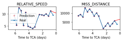
We now test the prediction. We take a single event, we remove the last CDM and try to predict it:

event=events_test[0]
event_len=len(event)
event_beginning=event[0:event_len-1]
event_evolution=model.predict_event(event_beginning, num_samples=100, max_length=14)
#we plot the prediction in red:
axs=event_evolution.plot_features(['RELATIVE_SPEED', 'MISS_DISTANCE'], return_axs=True, linewidth=0.1, color='red', alpha=0.33, label='Prediction')
#and the ground truth value in blue:
event.plot_features(['RELATIVE_SPEED', 'MISS_DISTANCE'], axs=axs, label='Real', legend=True)

Predicting event evolution
Time spent  | Time remain.| Progress             | Samples | Samples/sec
0d:00:00:08 | 0d:00:00:00 | #################### | 100/100 | 11.65