Plotting Functionalities#
In this tutorial, we shed some light on all the plotting functionalities of Kessler, and how to use them..
We tackle the following:
TLEs loading and plotting of their distributions
plot distributions from synthetically generated CDMs (these are generated using the probabilistic programming module, see the related tutorial
probabilistic_programming_module.ipynbfor a guide on how to use it)plot orbits from trace of synthetic CDMs
**Note**: A probabilistic program 'trace' is a record of all the random variables sampled in the program execution.
Let’s dive into these functionalities..
Imports#
import kessler
import dsgp4
import pickle
import numpy as np
First, let’s load the population#
This is here a file of TLEs (e.g. from Space-Track or Celestrack).. we use dsgp4 to handle TLEs
tles=dsgp4.tle.load('tles_sample_population.txt')
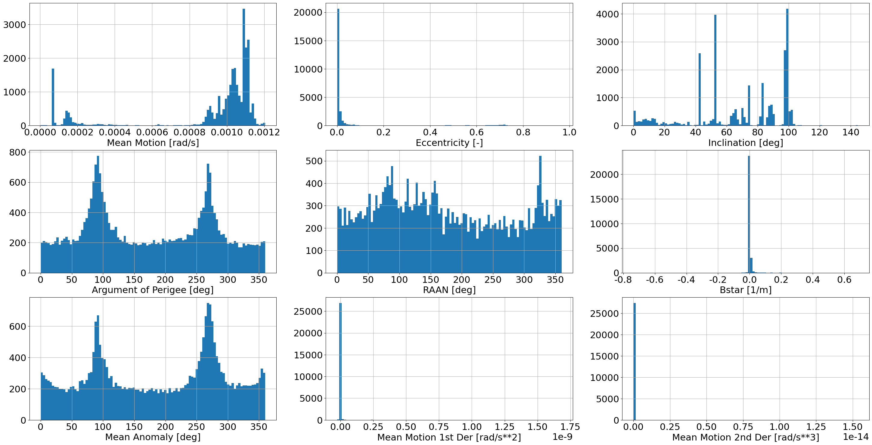
Let’s plot the distribution of the TLE elements from the loaded file
kessler.plot.plot_tles(tles)
Plotting priors from TLEs#
We can fit mixtures to the prior distribution and for instance use them as priors in the probabilistic programming module.
Here, we show how to display the prior :
priors=kessler.util.create_priors_from_tles(tles, mixture_components = {'mean_motion': 5, 'eccentricity': 5, 'inclination': 13, 'b_star': 4})
#we also extract the mean motion alues from the TLEs, to then have the minimum and maximum values for the mean motion priors (else the priors will be wide and you cannot see anything)
mean_motions=[el.mean_motion for el in tles]
kessler.plot.plot_mix(mix = priors['mean_motion_prior'],
                      min_val=np.min(mean_motions),
                      max_val=np.max(mean_motions),
                      log_yscale=True,
                      xlabel='Mean Motion',
                      figsize=(10,8),
                      linewidth=4.,
                      color='dodgerblue',
                      resolution=1000)
/Users/ga00693/miniconda3/envs/kessler/lib/python3.12/site-packages/torch/distributions/distribution.py:307: UserWarning: <class 'pyro.distributions.torch.MixtureSameFamily'> does not define `support` to enable sample validation. Please initialize the distribution with `validate_args=False` to turn off validation.
  warnings.warn(
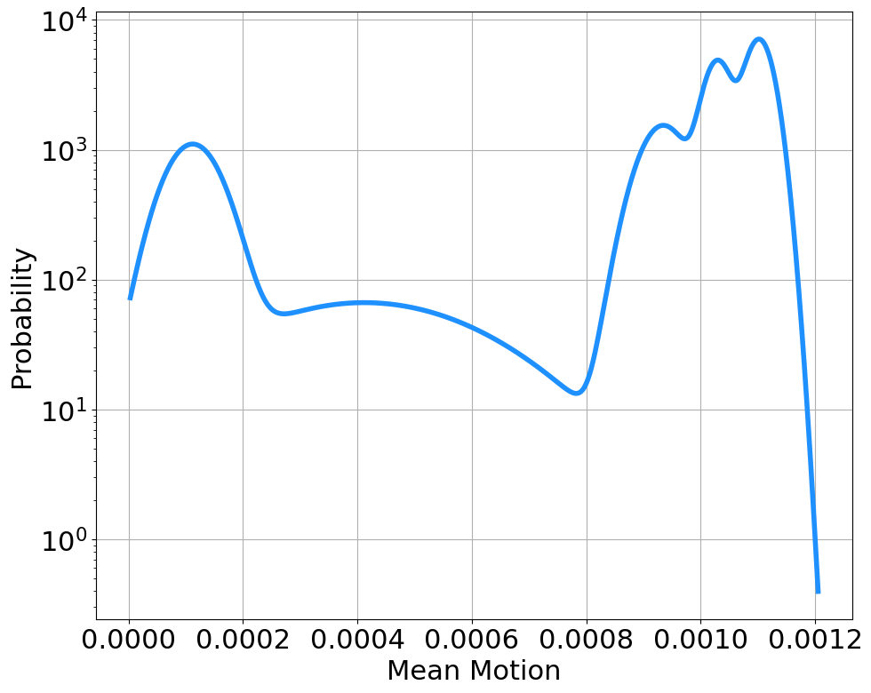
<Axes: xlabel='Mean Motion', ylabel='Probability'>
kessler.plot.plot_mix(mix = priors['inclination_prior'],
                      min_val=0.,
                      max_val=np.pi,
                      log_yscale=True,
                      xlabel='Inclination',
                      figsize=(10,8),
                      linewidth=4.,
                      color='darkorange',
                      resolution=1000)
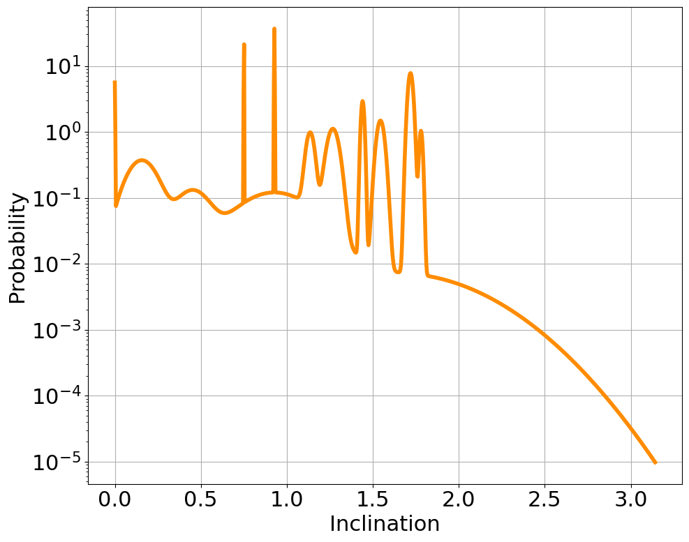
<Axes: xlabel='Inclination', ylabel='Probability'>
Plotting Orbit from Trace#
Let’s load the generated trace:
#save to pickle the trace:
with open('trace.pickle', 'rb') as f:
    trace = pickle.load(f)
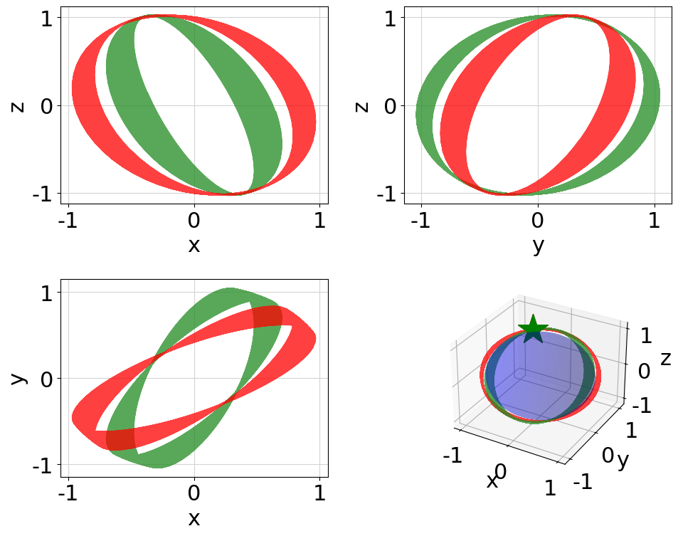
kessler.plot.plot_trace_orbit(trace=trace)
<Axes: xlabel='y', ylabel='z'>